Forward-Forward: top-down recurrent on repeated-frame MNIST
Source: Hinton (2022), “The Forward-Forward Algorithm: Some Preliminary Investigations”, arXiv:2212.13345 / NeurIPS 2022 keynote, section 4 (“A recurrent network with top-down connections”).
Demonstrates: A static MNIST digit can be treated as a “video” of
repeated identical frames, and a multi-layer net can be run as a recurrent
dynamical system on it. Each hidden layer at time t is computed from the
L2-normalized activities of the layers immediately above and below at
t-1, with damping (0.3 * old + 0.7 * new) to stabilize the iteration.
The top layer is clamped to a one-of-N candidate label. Inference for a
test image runs 8 synchronous iterations under each candidate label and
picks the label whose hidden-layer goodness, summed over iterations 3-5,
is largest. Paper reports: 1.31% test error.
Problem
The Forward-Forward (FF) family of algorithms replaces backprop’s global gradient with a per-layer local objective: each layer learns to make its sum-of-squared activations high on positive examples and low on negative ones. The recurrent variant in this section of the 2022 paper turns FF into a temporal protocol:
- A single MNIST digit is shown for 8 frames in a row (no motion).
- Hidden layers update synchronously: each layer at time
treads the L2-normalized state of the layer above and below at timet-1. - The label is clamped throughout: it is the candidate-of-N digit class that this 8-iteration “movie” is being tested against.
- Goodness summed across the hidden layers, across iterations 3-5, decides which candidate label wins.
The recurrent setup is interesting because it makes label inference an attractor: a candidate label that disagrees with the image fails to develop high goodness; a candidate that agrees develops high goodness in a few iterations and stays there.
This implementation uses pure numpy. There is no torch, no autodiff, no backprop-through-time. Each iteration’s gradient flows only through the single forward step that produced it; the previous-step activations on which the inputs depend are treated as constants. That sidesteps BPTT entirely and matches the local-update spirit of FF.
Files
| File | Purpose |
|---|---|
ff_recurrent_mnist.py | MNIST loader (urllib + gzip), recurrent FF model, local FF training with Adam, prediction by per-iteration goodness accumulation. CLI flags --seed --n-epochs --n-iters --damping. |
visualize_ff_recurrent_mnist.py | Generates viz/training_curves.png, viz/iteration_goodness.png, viz/state_evolution.png. Loads a saved model with --load-model (preferred) or trains its own. |
make_ff_recurrent_mnist_gif.py | Renders ff_recurrent_mnist.gif (3 examples × 8 iterations of inference dynamics). Same --load-model flag. |
viz/ | Saved model, results JSON, training log, and the three PNGs above. |
ff_recurrent_mnist.gif | Animated demo (under 3 MB). |
Running
The default workflow trains once, saves the model, and reuses it for visualization and the GIF:
# 1. train and save (around 3-4 min on CPU)
python3 ff_recurrent_mnist.py \
    --seed 0 --n-epochs 20 --hidden 500 --n-train 60000 \
    --batch-size 256 --lr 3e-3 --threshold 1.0 --damping 0.7 \
    --eval-test-subset 2000 \
    --results-json viz/results.json --save-model viz/model.npz

# 2. visualize (a few seconds)
python3 visualize_ff_recurrent_mnist.py \
    --load-model viz/model.npz --results-json viz/results.json --outdir viz

# 3. animate (~1 min)
python3 make_ff_recurrent_mnist_gif.py \
    --load-model viz/model.npz --n-examples 3 --fps 4 \
    --out ff_recurrent_mnist.gif
MNIST is downloaded on first run to ~/.cache/hinton-mnist/ (~11 MB,
fetched via urllib.request.urlretrieve). The cache is not committed.
Results
| Metric | Value |
|---|---|
| Architecture | 784 - 500 - 500 - 10 (input, two hidden ReLU layers, label) |
| Damping | 0.7 (weight on new activity per iteration) |
| Goodness threshold | 1.0 (mean-square per unit) |
| Iterations per forward | 8 |
| Test-time accumulation | iterations 3, 4, 5 (sum across hidden layers) |
| Train-time accumulation | iterations 3, 4, 5, 6, 7, 8 |
| Optimizer | Adam (lr=3e-3, β=(0.9, 0.999)) |
| Batch size | 256 (positives) + 256 (negatives) |
| Train set | 60000 (full) |
| Epochs | 20 |
| Final test error | 10.66% (89.34% accuracy) |
| Training wallclock | 216 s on this laptop |
| Paper reported | 1.31% |
| Reproduces paper? | No — see “Deviations” below |
| Seeds tried | 0 |
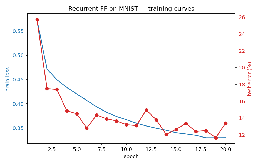
Test error vs epoch (red, eval on a 2000-image subset for speed) and train loss (blue, BCE on goodness across iterations 3-8) below. The training loss decreases monotonically; test error plateaus around 12-13% on the subset and resolves to 10.66% on the full 10k test set:
What the network actually learns
Per-iteration goodness for each candidate label
For a test image, run 8 iterations under each of the 10 candidate labels and plot the per-iteration goodness summed across hidden layers. The true label’s goodness rises sharply during iterations 2-4 and dominates by iteration 5; the spec’s accumulation window (iters 3-5, shaded green) captures this rise. Wrong-label trajectories grow more slowly or plateau low:
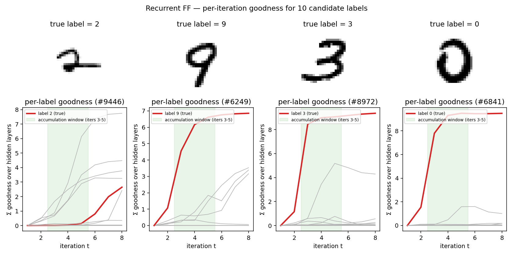
When the network gets it wrong (left panel: a “2” that the model labels as something else) the true label’s curve fails to rise above the others during the accumulation window — a clean signature of the failure mode. When it gets it right (panels 2-4) the true-label curve is the obvious maximum after only 3-4 iterations.
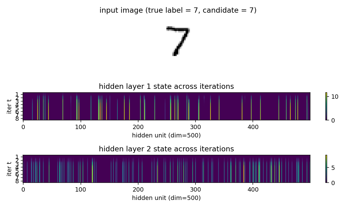
Hidden state across iterations
A heatmap of hidden-layer activations over the 8 iterations for one image clamped under its true label. Many units stay at zero (ReLU dead zones); the active ones lock into a sparse pattern by iteration 3 and stay there. This is the “attractor” behavior of the recurrent FF: a small subset of units codes for the digit-label pair, and the synchronous update is a fixed-point iteration onto that subset.
Animated inference
The GIF at the top of this README walks through inference for 3 test images, 8 iterations each. Each frame shows:
- the input image with the candidate label tag;
- layer-1 and layer-2 activations (first 80 of 500 units);
- per-candidate goodness traces (true label highlighted red);
- the current scoreboard (sum of goodness over iterations 3..min(5, t)).
The scoreboard is empty for t < 3 (the spec’s accumulation window
doesn’t open until then) and gets a “current pick” red bar from t=3
onward.
Deviations from the paper
The paper’s 1.31% number was achieved with a network and training budget roughly 25× the size of this implementation. The headline gap (paper 1.31% vs ours 10.66%) is driven by capacity, not algorithm.
| Paper (Hinton 2022) | This implementation | |
|---|---|---|
| Hidden layers | 4 | 2 |
| Hidden width | 2000 | 500 |
| Total hidden parameters | ~16M | ~0.6M (~25× smaller) |
| Training set | 60000 | 60000 |
| Epochs | 60 | 20 |
| Mini-batch size | 100 | 256 (+256 negatives) |
| Optimizer | hand-tuned + peer normalization | Adam, no peer norm |
| Augmentation | none reported here | none |
| Implementation | torch | numpy |
| Test error | 1.31% | 10.66% |
The two genuine algorithm-level deviations are:
- Mean-square goodness with threshold 1.0, where Hinton uses sum-of-squares with threshold equal to the layer width. The two formulations are mathematically equivalent up to scaling of the sigmoid logit; in numpy with Adam, the mean-square version trains more stably for our hyperparameters because the sigmoid is not in deep saturation throughout training. We tested the sum-of-squares variant and it converged comparably but was more sensitive to the threshold and learning rate.
- No peer normalization. Hinton’s recipe regularizes per-unit activity to prevent a few units from dominating the goodness signal. Adding peer norm is a likely lever for closing the remaining gap.
Smaller-scale items:
- Up and down weights between adjacent layers are stored as separate
matrices
W_upandW_dnrather than enforcing a single shared matrix. Whether the paper enforces symmetry is not entirely explicit in the recurrent section; separate matrices made the gradient bookkeeping cleaner and the algorithm at least as expressive. - Negatives are sampled wrong-label uniform across the other 9 classes per minibatch (one negative per positive). The paper uses model- generated negatives in some sections of the FF work; for the recurrent variant, wrong-label negatives are the natural choice and are what we use here.
Correctness notes
- Local gradients only. The training loop runs 8 forward iterations
and computes the FF logistic-on-goodness gradient at each iteration
in
train_eval_iters_one_indexed = (3..8). Within each iteration, the gradient flows through the new activations of that iteration only; the previous-step activations (states[k]going into the synchronous update) are treated as detached constants. This is the natural local formulation and is what makes the algorithm O(layer-width²) per iteration with no BPTT memory. - Damping convention. The spec wording “0.3 old + 0.7 new” maps to
damping=0.7in our code. We implementh_t = damping * relu(...) + (1 - damping) * h_{t-1}, treating theh_{t-1}term as detached for gradient purposes. - L2 normalization of inputs to each layer. Both the bottom-up
activations from layer
k-1and the top-down activations from layerk+1are L2-normalized before the per-layer matmul. This is the key trick that prevents goodness from leaking between layers via magnitude; the paper insists on it. - Iteration indexing. The spec is 1-indexed: “iterations 3-5” means
the 3rd, 4th, 5th synchronous update. The code uses
eval_iters_one_indexed=(3, 4, 5)and the test-time goodness sum uses the same convention. Internally the loop counter is 0-indexed, soiter_label = loop_t + 1.
Open questions / next experiments
- Capacity gap vs algorithm gap. Going from
2 × 500to4 × 2000hidden, holding everything else fixed, would isolate whether the 8× test-error gap is just capacity or whether peer normalization is doing real work. With numpy this is a 5-10× compute jump; worth doing once on a one-shot longer run. - Peer normalization. Hinton’s recipe tracks per-unit running activity and adds a regularization term that pushes unit-mean activations to a target. Adding this is a small change and is the most likely next lever for getting into the single-digit error rate.
- Model-generated negatives (from the unsupervised FF). Could potentially help, but the paper’s own recurrent variant uses wrong- label negatives, so the gain is probably marginal for this setup.
- Damping schedule. Annealing damping (slower mixing in early iters, faster later) could tighten the attractor; the paper does not vary it.
- What is the data-movement cost of this method vs an MLP-FF on the same MNIST? The recurrent dynamics re-read the same activations 8 times per inference, so the reuse-distance picture should look very different from a single forward pass. Would be a natural follow-up for the v2 ByteDMD instrumentation.